How a small style-LoRA project makes its decisions — the calibrated gates, the controlled A/Bs, the metric design — using three illustration sub-styles (painterly, storybook-sketch, ink-wash) as the worked example. Training and eval ran on 8× A100 (80 GB). Every figure and number is read back from reports and embedding/weight files saved at generation time, so the same inputs reproduce them.

0. The approach

The working rule is to replace every “looks good” with a measured decision against a per-dataset calibrated threshold in a single feature space, and to treat each knob as a controlled A/B with a pre-declared adopt criterion and a known noise floor. The failure mode this guards against is the invisible one — by eye you can’t tell underfit from bad data from wrong-base-model — so nothing is adopted because it “should” help; it’s adopted because a number cleared a bar set before the run.

Three principles run through everything:

1. One feature space, end to end. The same embedder (DINOv2) is used for data triage, coherence auditing, and final eval. “Passes curation” and “passes eval” therefore measure the same thing — no metric mismatch between the gate you select data with and the gate you grade output with.
2. Calibrated thresholds, not guessed absolutes. Every gate is a percentile of the reference set’s own intra-set distribution, not a magic number like 0.75. Tight datasets auto-tighten; loose ones auto-relax.
3. Measure before you spend. Coherence, distribution drift, and per-image exposure are all checked as a pre-flight that can halt the train — detection moves to before the 25-minute A100 burn, not after.

---

1. Why DINOv2, not CLIP

The whole stack is built on DINOv2 embeddings. CLIP is semantic (trained on image–text pairs, so it encodes “what is depicted”). DINOv2 is self-supervised on visual features, so it weights medium / texture / surface / style far more heavily than CLIP does — much closer to the axis a style LoRA is trying to lock.

It is style-dominant, not style-pure. DINOv2 is not invariant to subject identity, composition, or spatial layout; the embedding stays entangled with all three. So cosine-to-centroid is a defensible proxy for style only as a relative measure with the subject distribution held roughly constant — for clustering, outlier detection, and ranking — not as an absolute, subject-agnostic “is this on-style” verdict. §5 engineers that constant-subject condition deliberately (eval subjects drawn from the training distribution) and its stress test shows the metric scoring subject distance the moment the condition breaks. For a project where “style is the product,” that style-dominant axis is still the right thing to gate on where CLIP’s semantic axis would punish the very subject variety the references are built for. CLIP scores are still computed and reported for visibility, but they never gate a decision.

This choice is upstream of everything: it’s why the gates mean something, and it’s what makes a deliberate subject-variety reference set possible without the metric punishing that diversity.

---

2. Data tier discipline (the input contract)

Two physically separate tiers, enforced by a rule and a pre-tool hook:

• The active training set — curated, one folder per sub-style. Training reads only from here. The set of folders that exists is the sub-style list, discovered at runtime (no central registry; adding a sub-style is a single-folder operation).
• The staging / reserve pool — collected, not curated. Never read by training.

They are not interchangeable: loading from staging would skip the manual eval gate that decides whether an image represents the sub-style, silently contaminating the LoRA — and the only fix for a contaminated LoRA is a re-train. The promotion path from staging to active is the only sanctioned route and runs through a classifier with a human review step:

classify (DINOv2 cosine vs each folder centroid) → CSV report → human review → copy in (never a blind move)

A per-label target count grows a folder toward N total in a single pass without manual top-K selection. Floor: 20 images before a folder can train at all.

Concretely, promotion is classifier-mediated, human-reviewed, and append-only, gated on a similarity threshold — and the threshold itself is calibrated (next section) rather than fixed by hand.

---

3. The calibrated coherence gate (curation as a pre-flight, not an afterthought)

Reference-set coherence — “is this folder internally consistent enough to define one style?” — is checked before training rather than as an eval-time question answered post-training. It runs as a mandatory pre-train gate, invoked automatically by the trainer; a non-zero exit halts the train.

It computes the DINOv2 intra-set distribution of the folder — every image’s cosine to the set centroid — and reports the full percentile spread (Table 1):

substyle	n	min	p10	p25	p50	p75	p90	max	mean	std	verdict
ink_wash	109	0.555	0.615	0.658	0.703	0.746	0.776	0.855	0.701	0.064	PASS

Two things fall out of this one audit:

1. A PASS/FAIL on absolute mean + p25 floors — does this folder cohere at all?
2. The per-folder p25 becomes the calibrated runtime threshold used downstream by both the classifier and the eval grid. The folder defines its own on-style bar.

The same numbers drive a human-in-the-loop curation pass. An interactive view lays out every reference thumbnail with its cosine-to-centroid, the intra-set histogram with the mean and the p25/p10 gates drawn on it, and the caption-diversity verdict — so trimming the weakest refs is a ranked, data-driven edit against the exact distribution the automated gate will enforce, not a hunt by eye. The thumbnail grids double as the first concrete look at the three sub-styles themselves: ink_wash’s limited-palette brush-and-wash, painterly’s saturated gouache, storybook_sketch’s pen-and-ink storybook linework. Each panel shows that folder’s own thumbnails, its intra-set histogram, and its gates — the per-folder calibration of the previous section, from the operator’s side (Figures 1–3):

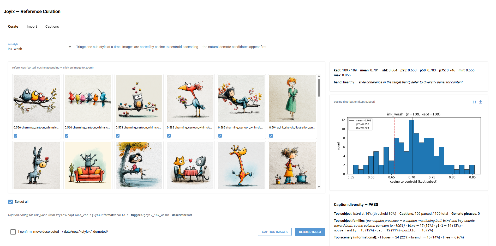
Reference-curation view for ink_wash: thumbnails labelled with DINOv2 cosine-to-centroid, the intra-set histogram with mean and p25/p10/p5 gates, and the caption-diversity panel.

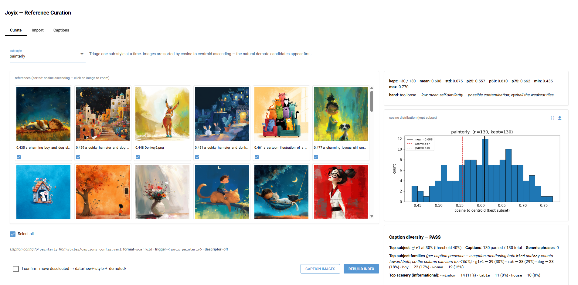
Reference-curation view for painterly: thumbnails labelled with cosine-to-centroid, the folder’s intra-set histogram with mean and p25/p10/p5 gates, and a caption-diversity PASS.

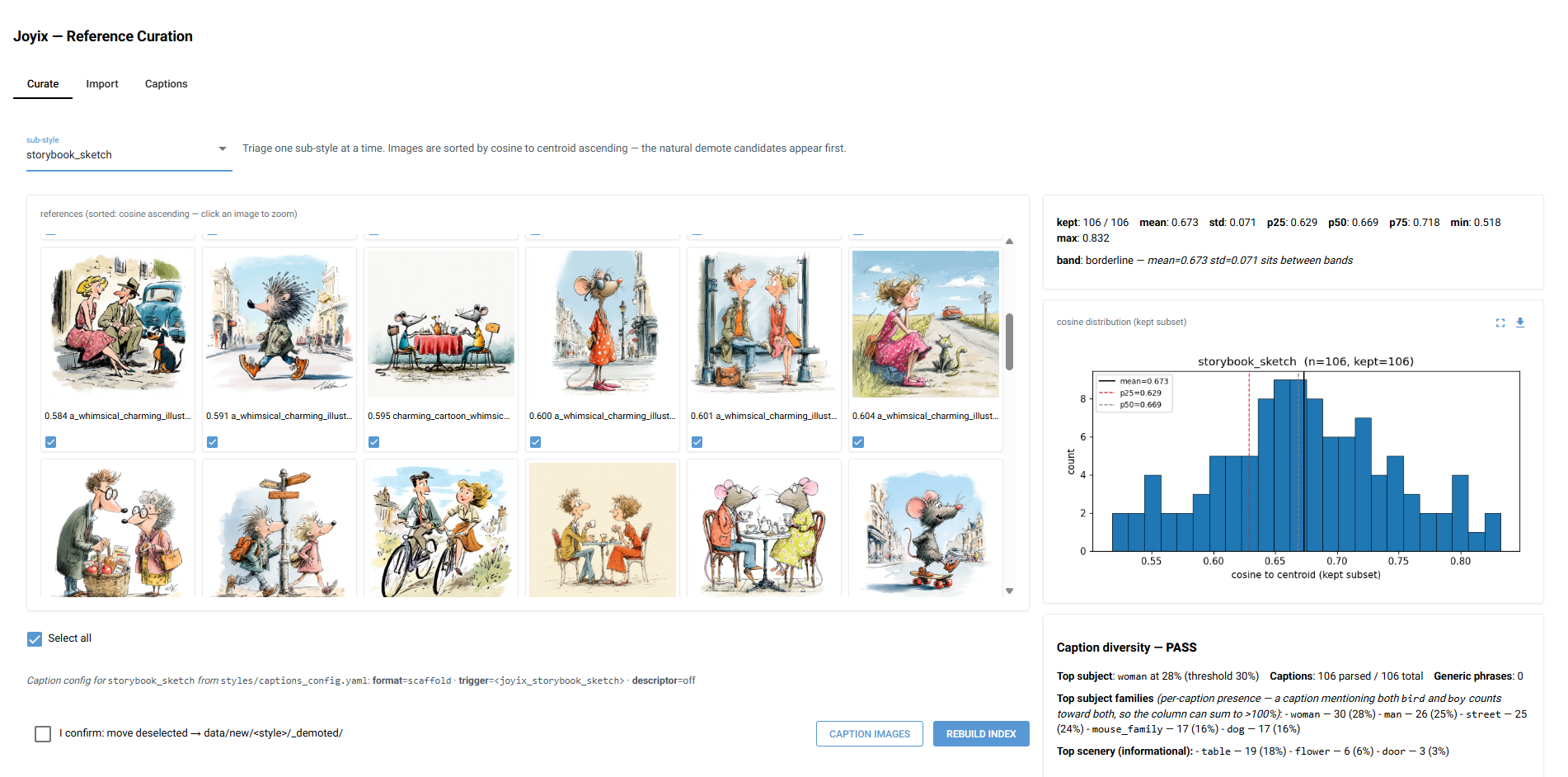
Reference-curation view for storybook_sketch: thumbnails labelled with cosine-to-centroid, the intra-set histogram with mean and p25/p10/p5 gates, and a caption-diversity PASS.

The third panel — caption diversity — is a second curation axis, orthogonal to coherence. Coherence asks is this folder one style? (tight in DINOv2 space); caption diversity asks whether the subjects are varied enough. It reads the kept images’ bare-subject captions, counts how often the single most-common subject family appears, and flags the folder when that share exceeds a per-folder threshold. The two gates pull in deliberately opposite directions — coherence wants the set tight in style, caption diversity wants it broad in subject — because a folder that is coherent and subject-narrow (mostly the same animal, say) risks teaching the LoRA the recurring subject instead of the style. Surfacing both live means a trim that tightens style can’t quietly narrow subjects unnoticed; §4 covers the captioning side, and §9 the related out-of-domain wall.

Calibration in the wild: three styles, three different gates

The three sub-styles land at materially different calibrated p25 gates — not because anyone chose them, but because their reference sets have different natural self-similarity (Table 2):

sub-style	ref set	calibrated gate (p25)	reading
painterly	~130 imgs	0.556	loosest refs → lowest bar
storybook_sketch	~106 imgs	0.629	mid
ink_wash	109 imgs	0.658	tightest refs → highest bar

A ridgeline reader renders this as one KDE per folder of every image’s cosine to its own centroid, with the folder mean (red) and the calibrated p25 gate (dashed) marked (Figure 4):

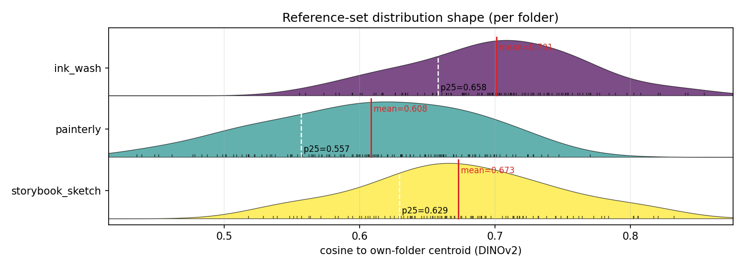
Per-folder ridgeline of DINOv2 cosine-to-own-centroid; each curve is annotated with its mean (red) and its calibrated p25 gate (dashed). The three ridges sit at visibly different places — the calibration argument in one picture.

The picture is the calibration argument. The three ridges sit at visibly different places on the x-axis — painterly (mean 0.608) is shifted a full ~0.09 left of ink_wash (mean 0.701), with storybook_sketch (0.673) between them — and each folder’s dashed p25 tracks its own ridge, not a shared line. The rug ticks along each baseline are the individual reference images, so you can also read shape (skew, any bimodality) straight off the plot during curation.

The 2-D view: are the sub-styles actually separable?

The ridgeline is the 1-D marginal of each folder’s embedding distribution. The 2-D companion projects the full 768-d embeddings of all folders into one shared space and scatters them coloured by folder — the “view the dataset in latent space” picture (Figure 5). It reads the same cached embeddings (no GPU, no re-embed), so it’s a pure reader on a warm cache.

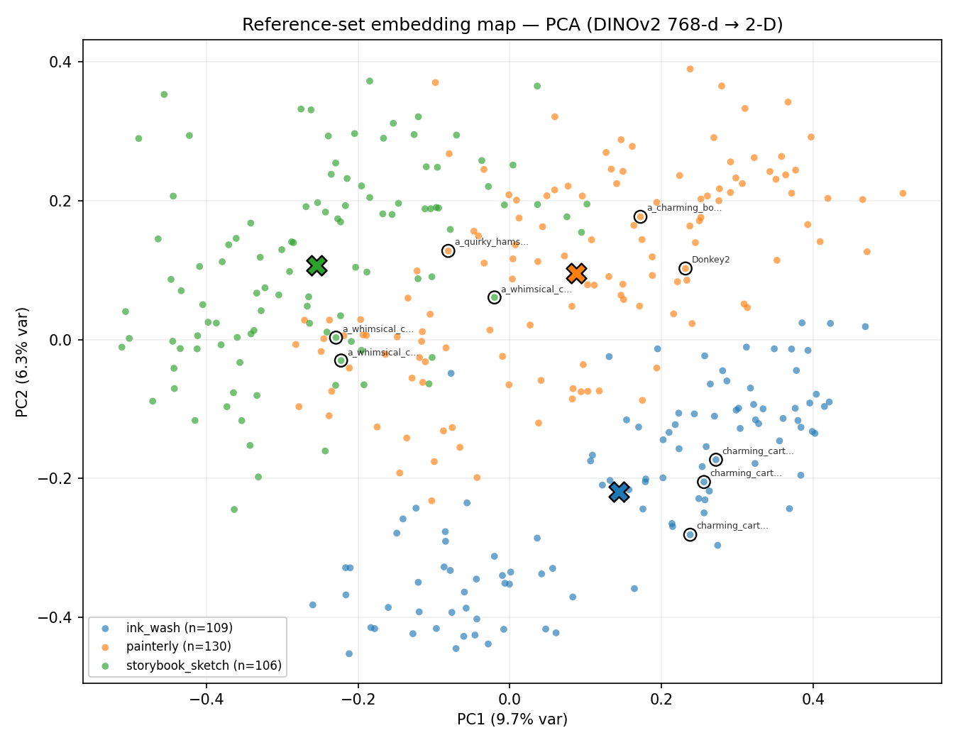
PCA projection of the DINOv2 embeddings, one point per image coloured by folder, with folder centroids (X) and the lowest-cosine curation outliers ringed. The two axes capture only ~16% of the variance, so overlap understates separation.

The three folder centroids (X) sit in distinct regions — storybook_sketch top-left, painterly centre, ink_wash bottom-right — and the ringed points are the curation outliers (lowest cosine to their own centroid), now located spatially. Caveat: the two PCA axes capture only ~16% of the 768-d variance, so visual overlap in the projection understates separation. The honest, projection-independent read is the separability table (Table 3) computed alongside — each folder’s mean cosine to its own centroid vs the nearest other centroid, in full 768-d:

sub-style	mean own-centroid cos	nearest other	margin	nearest
ink_wash	0.701	0.557	+0.144	painterly
painterly	0.608	0.484	+0.125	ink_wash
storybook_sketch	0.673	0.492	+0.181	painterly

Every margin is positive — the average reference image is markedly closer to its own centroid than to any neighbour, so the three sub-styles are empirically well-separated under cosine geometry (which is what licenses treating them as distinct sub-styles and trusting the per-folder gates). This is separation in the centroid-cosine sense — positive mean margins plus the projection above — not a formal proof of linear separability: the PCA view captures only ~16% of the variance and the margins are over folder means, not a guarantee that a single hyperplane cleanly partitions every individual image. Read it as strong empirical separation, not a theorem. The projection is PCA by default; a t-SNE / UMAP variant is also available.

A single absolute threshold (an earlier 0.70 / 0.75 / 0.90 guess) would have been simultaneously too strict for painterly and too lax for ink_wash — and in fact some folders’ own references could not clear the absolute bar their refs would need to clear. Per-folder p25 fixes that by construction: it auto-tightens a coherent folder and auto-relaxes a looser one. The number is read from the dataset, never hardcoded — a hardcoded count or threshold is a silent drift surface.

The gate also surfaces the weakest refs (lowest cosine to centroid), so curation is a ranked, data-driven trim rather than a hunt.

---

4. Caption discipline: build, don’t author

Captions are a derived build artifact, not hand-written training text. The principle: the human edits a bare subject phrase per image; the full training caption is generated forward from that subject by a single composer and is never hand-edited.

bare subject  →  forward composer  →      composed caption (what the trainer reads)
(human-edited)   (applies envelope ONCE)  (NEVER hand-edited)

• The source of truth is a bare subject phrase per image — no trigger, no scaffold, no descriptor.
• The composed caption (`, , `) is generated forward by a single composer. The train pre-flight *verifies* each on-disk caption equals what `(subject + config)` composes to — so train / preview / inference **cannot drift** by construction.

Three knobs (caption format, whether the trigger token is present, whether a fixed style descriptor is appended) have a deliberate two-source split:

• A live config drives caption authoring and new trains.
• A per-LoRA frozen snapshot, written next to each checkpoint at train time, drives inference — it freezes the three knobs and the resolved envelope text (descriptor string + scaffold anchors). Editing the live descriptor later does not change how an already-trained LoRA is prompted. This kills the drift surface where inference reads a config that’s been edited since training.

The transferable captioning finding

Caption what you want to VARY; omit what you want the TRIGGER to own.

Validated by a clean A/B on ink_wash (FLUX, matched gen-seed, descriptor presence confirmed in the training log): putting the textured-paper descriptor into training captions regressed the result (seed_42 0.655 → 0.612, −0.043; seed_77 0.573 → 0.560), because the texture is constant across the set — it is the style, so it belongs to the constant trigger token, not restated in descriptor words. A constant phrase in every caption carries no discriminative gradient; it just splits “always-on style” credit between two text loci and weakens both. The strong ~0.67 result came from the descriptor at inference only. (There’s an architectural reason this bites harder on FLUX — see §11.)

Subject-narrowness is audited separately: a folder FAILs when its single most-common subject family exceeds a per-folder threshold — raised where subject-narrowness is intentional (a human-figure or single-character set is narrow by design, not by accident). The three folders pass this audit, yet still hit an out-of-domain wall in §9 — so the single-dominance check is necessary, not sufficient: the held-out novel-subject tail can collapse even when no one subject dominates the training set. The held-out diversification prompts are the probes that expose that wall (§5’s diversity tail), not a mitigation that was applied to the folders.

A public dataset’s captions are unvalidated input

The build pipeline is faithful by construction, which cuts both ways: a wrong bare subject propagates straight into the training signal — and, since the eval subjects are derived from the same source (§5), into the eval prompts too. So the human-review gate sits on the subject tier, not the composed output, and it can’t be skipped for an auto-captioned set.

That holds doubly for a dataset pulled from a public hub. Being on a model hub says nothing about caption fidelity — the dataset ships whatever its auto-captioner emitted at upload. The standard naruto-blip-captions set (the nrtcel stress test in §5) was captioned with an early BLIP: naruto_0002, a masked creature, is labeled “a man with a red hair and a black shirt” — not partially off, entirely wrong. A current BLIP2 re-caption fixes some cases, mislabels others, and folds the constant style word (“anime”) into ~60% of subjects — which the caption-what-varies rule above says to strip anyway. An automated style-word strip clears that constant-word layer; subject accuracy still needs human (or strong-VLM-then-human) review before the source can be trusted.

---

5. The eval metric (graded the same way data is gated)

The eval grid is scored with the same DINOv2 embedder, against the same per-folder calibrated gate. Five non-obvious design choices:

1. Mean, not rate. Generations cluster right at the p25 gate, so the on-style rate is a knife-edge coin-flip (it can swing 47%↔73% between adjacent checkpoints while the mean barely moves). That instability is partly a metric-discontinuity artifact, not model variance: the rate is a hard-thresholded count over a continuous score distribution, so when the mass piles up on the gate, a sub-noise shift tips many samples across the line at once — the threshold’s position relative to the distribution inflates the rate’s variance independently of any change in the weights. The mean is a smooth functional of the same scores and stays stable. Select and compare on the mean; report the rate.
2. Best-checkpoint, not final. The step budget is uniform and arbitrary; intermediate checkpoints are retained precisely to do held-out selection. Reading final penalizes whichever style peaked earlier (painterly peaks ~step3000 at 73% and decays to 49% by final). Best-checkpoint selection picks the best step per style/seed on the mean.
3. In-domain prompts derived from the training distribution. Because DINOv2 conflates style + subject, an off-domain subject scores low even if rendered perfectly on-style. So eval subjects are materialized from the sub-style’s own training captions (de-duped + diversity-filtered). This holds the subject distribution roughly constant so the residual cosine signal is style-dominant — a style comparison rather than a subject test. (The entanglement is controlled, not removed: composition still varies per generation, which is why the verdict rides on the mean and the gate, never a single image’s score.) Eval prompts are committed (versioned against the dataset state), never hardcoded.
4. The diversity tail is scored separately. 5 held-out novel-subject prompts are graded at the relaxed p10 gate in their own report — not folded into the main number at p25 (which would double-penalize out-of-domain subjects and understate in-domain fidelity by ~5 pp).
5. Memorization probe. Max nearest-reference cosine vs the ref set’s own p99 nearest-neighbour bar — distinguishes “learned the style” from “recalled a training image.”

Noise band as a first-class object: the run-to-run band is std ≈ 3–6 pp (n=2 seeds). A gain counts as real only if it exceeds ~2σ (~12 pp) on the rate or moves the best-checkpoint mean clearly over the gate. Every adopt decision has a pre-declared threshold: mean must clear the gate by > 0.02.

When the conflation bites: a standard-dataset stress test

Design choice #3 is easy to assert and easy to under-weight. Training a standard public dataset — naruto-blip-captions (a canonical fine-tuning example), run here as a deliberately non-word sub-style nrtcel so the trigger carries no base-model prior — makes the conflation impossible to miss.

The SDXL LoRA trains cleanly: the best checkpoint scores mean 0.666, rate 73%, +0.073 over its gate (0.59) — the highest mean of any sub-style here. (It also plateaus mid-run: the mean reaches a ~0.65–0.67 shelf by ~step3000 and stays there for the rest of the 11k-step run — peak step5000, and steps 7000–11000 never beat it — so the back half of the budget added nothing; a redundant, low-variance style locks in fast.) But the rate stalls at 73%, and every low scorer is a non-portrait subject — scenery, animals, full-body scenes — while every high scorer (0.77–0.79) is a character close-up. That is not a style failure (Figure 6):

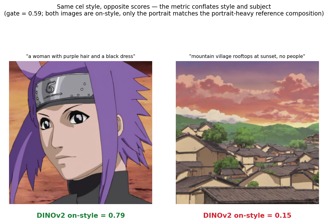
Same LoRA, same style, opposite scores: a character portrait scores 0.79, a peopleless cel-shaded landscape 0.15. The metric is scoring subject distance, not style — why the verdict rides on the mean, never a single image.

Both images are unmistakably on-style; the portrait scores 0.79, the landscape — a clean cel-shaded establishing shot — scores 0.15. The reference set is almost entirely character portraits, so a wide peopleless landscape sits far from that centroid in DINOv2 space whatever its style. The metric is scoring subject distance, exactly as choice #3 warns — and it bites hardest here precisely because the references are compositionally uniform, so the in-domain rate understates the LoRA’s real style transfer (it renders scenes on-style better than a portrait-built centroid can credit).

Same lesson as §9’s diversity wall, sharpened: rate is a subject-coverage signal as much as a style one — which is why the mean (choice #1) and the separately-graded diversity tail (choice #4) are the honest numbers, and a lone rate threshold is never a verdict by itself.

---

6. Experiment design

• Dedicated results tree per experiment — each experiment’s checkpoints and eval outputs land under their own labelled folder, so every A/B is clean and identifiable from the path alone.
• Two failure modes are tracked separately and never conflated:
  • In-domain underfit (mean below gate) → recipe levers (rank, LR, scheduler, TE, descriptor, set size).
  • Out-of-domain generalization (0% diversity on novel subjects) → data levers (reference + caption subject diversity). No recipe knob touches this.
• Seed-vs-noise separation. Because a single training seed can land ±0.085 apart on a small set, a generation-seed sweep (gen-seeds × trained-seeds) separates training-seed effect (genuine weight quality) from eval noise-draw variance. The ink_wash FLUX finding: the ~0.085 training-seed gap persists across all gen-seeds (~4× the ~0.02 eval noise) → best-of-N training seeds is mandatory, not optional.
• Common-bar cross-scoring. A reader re-embeds the generated eval images against any chosen reference centroid + p25, so two LoRAs scored against different reference sets can be compared on one common bar.
• Pure-reader analysis. Every eval run stores its per-image scores, and all the analysis (best-checkpoint selection, seed summaries, the gen-seed sweep, cross-scoring) re-reads those stored scores rather than re-generating — so a metric change re-grades old runs without re-rendering a single image.

---

7. Data integrity & texture preservation

The model never trains on the reference PNGs directly — it trains on their VAE round-trip, read from a per-image latent cache. Two links therefore sit between the curated references (§3) and the trained weights, and the rest of this doc doesn’t otherwise check them: what the model actually ingests (the VAE encode→decode of each reference) and whether the cached inputs are clean (no corrupt, anomalous, or stale-from-another-base latents). Both are verifiable up front rather than inferred from a disappointing result, and both are measured in the same DINOv2 feature space the gates use. The two checks below cover them: texture preservation (the VAE round-trip) and data integrity (the cached latents). Opening the LoRA’s weights is a separate question, taken up in §8. Where all of these checks sit among existing interpretability and data-validation tooling is mapped in §13.

Texture preservation: the VAE round-trip

The diffusion model never trains on the reference PNG — it trains on the VAE round-trip of it (the trainer caches the VAE-encoded latents per image). For a texture-defined style like ink_wash, an obvious suspect for the ceiling is “the VAE smooths the ink / flattens the paper grain before the LoRA ever sees it.” That’s a verifiable claim, not a thing to assume either way. A latent-decode reader decodes the cached latents back to RGB (the model-space inverse of the VAE encode) and compares each to its original — visually and in the same DINOv2 space the gate uses (Figure 7):

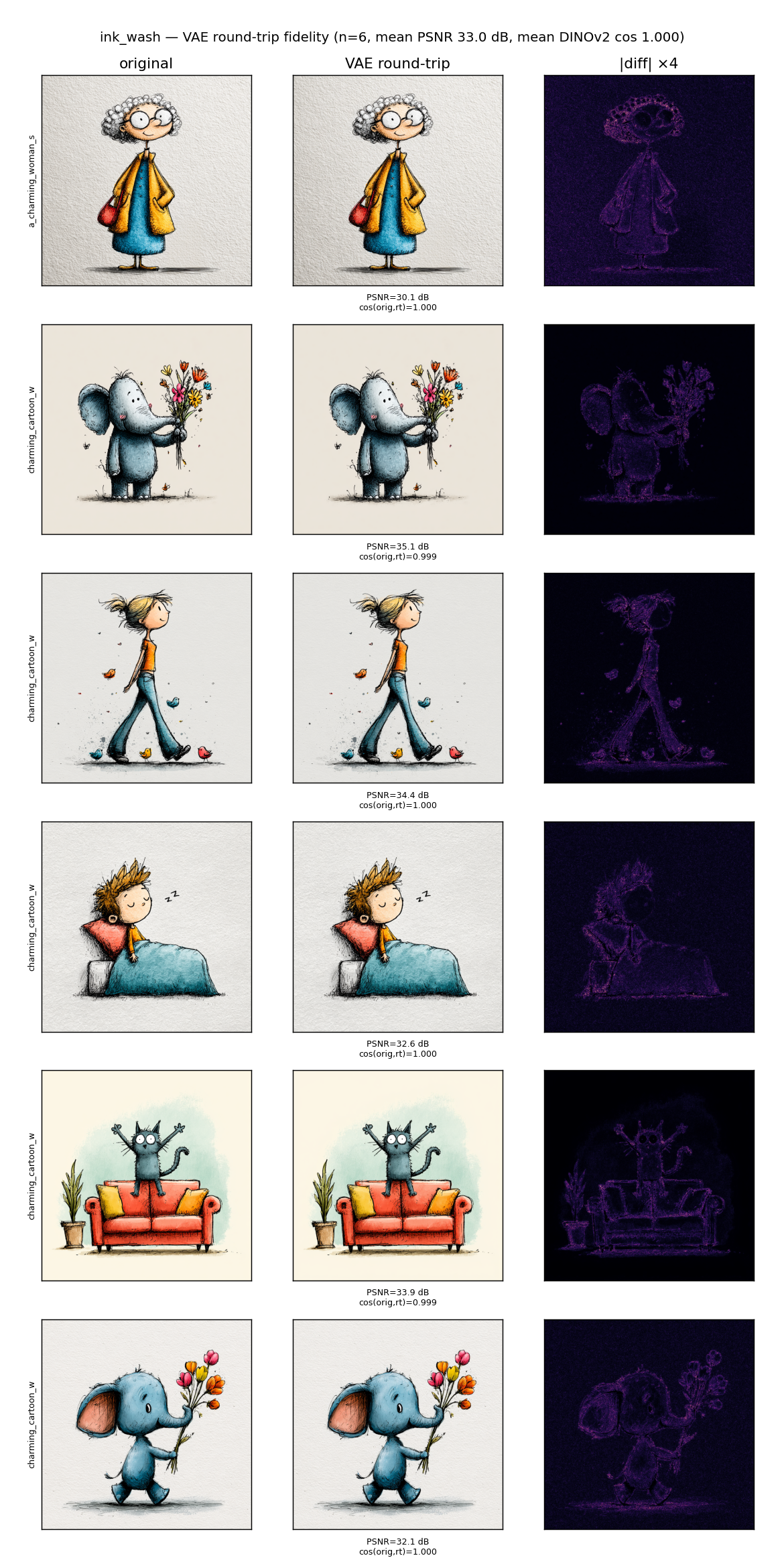
ink_wash VAE round-trip (FLUX): original, round-trip, and amplified diff. Visually identical (PSNR 33 dB, cosine 0.9995); residue only on the finest ink-line edges.

Result: mean PSNR 33 dB, mean DINOv2 cosine(original, round-trip) = 0.9995 — the round-trip is indistinguishable from the original in the gating feature space, the amplified diff showing only faint residue on the highest-frequency ink edges. That scopes the conclusion rather than settling it outright. Both metrics are relatively insensitive to the very signals a texture-defined style leans on — micro-texture statistics, frequency-domain content, brushstroke stochasticity — PSNR being a low-frequency-weighted global MSE, and DINOv2 the same style-dominant embedding §1 cautions against reading as texture-complete; and the residue sits exactly on the high-frequency ink edges where that signal lives. So the round-trip cannot be claimed to preserve texture in full. What it does establish is narrower and sufficient: whatever the VAE discards is invisible in the same DINOv2 space the gate scores in, and so cannot be the cause of a DINOv2-measured ceiling. The VAE is therefore unlikely to be the dominant bottleneck, but cannot be fully eliminated as a contributor to texture loss — the ~0.67 ceiling is, to the metric that defines it, downstream of the LoRA’s fit rather than input fidelity, established in the gate’s own feature space before reading any training result.

The VAE loss is base- and texture-dependent

That FLUX round-trip is the best case. Re-running the same probe per base and per style — the SDXL workhorse alongside FLUX — shows input fidelity is not a single number but a function of two compounding factors (Table 4):

style (content)	FLUX PSNR / cos	SDXL PSNR / cos
nrtcel (cel-shaded, flat)	41.3 dB / 0.9985	42.1 dB / 0.9954
painterly (brushwork)	31.8 dB / 0.9997	26.7 dB / 0.9958
storybook_sketch (ink line)	31.1 dB / 0.9996	23.0 dB / 0.9946

PSNR here is measured in shared RGB pixel space against the identical source image, not in latent space — so the FLUX↔SDXL gap across a row is a like-for-like reconstruction-fidelity comparison, and the channelization difference (16-ch vs 4-ch) is its cause, not a unit mismatch. Absolute dB down a column is a different matter: it is content-dependent (a flat cel-shaded frame scores high almost for free), so the cross-style differences are a trend, not a cross-style fidelity ranking.

Two factors multiply:

• VAE channel capacity (the base). FLUX’s VAE encodes to a 16-channel latent; SDXL’s to 4 channels (both at 8× spatial downsampling). A quarter of the channel capacity reconstructs high-frequency detail far less faithfully, so for the same image SDXL’s round-trip PSNR is lower.
• Content frequency (the style). A cel-shaded set — flat colour, hard edges, little stochastic texture — is reconstructed almost perfectly by both VAEs (41–42 dB), and SDXL’s capacity shortfall never bites, so the two bases converge. Brushwork and dense ink linework are high-frequency everywhere, so both bases lose more and the gap widens, because the missing SDXL channels hurt most exactly where the signal lives. storybook_sketch — finest linework, highest frequency — is the worst case: SDXL drops to 23 dB, an 8 dB gap, the amplified diff lighting up the entire line structure (Figure 8).

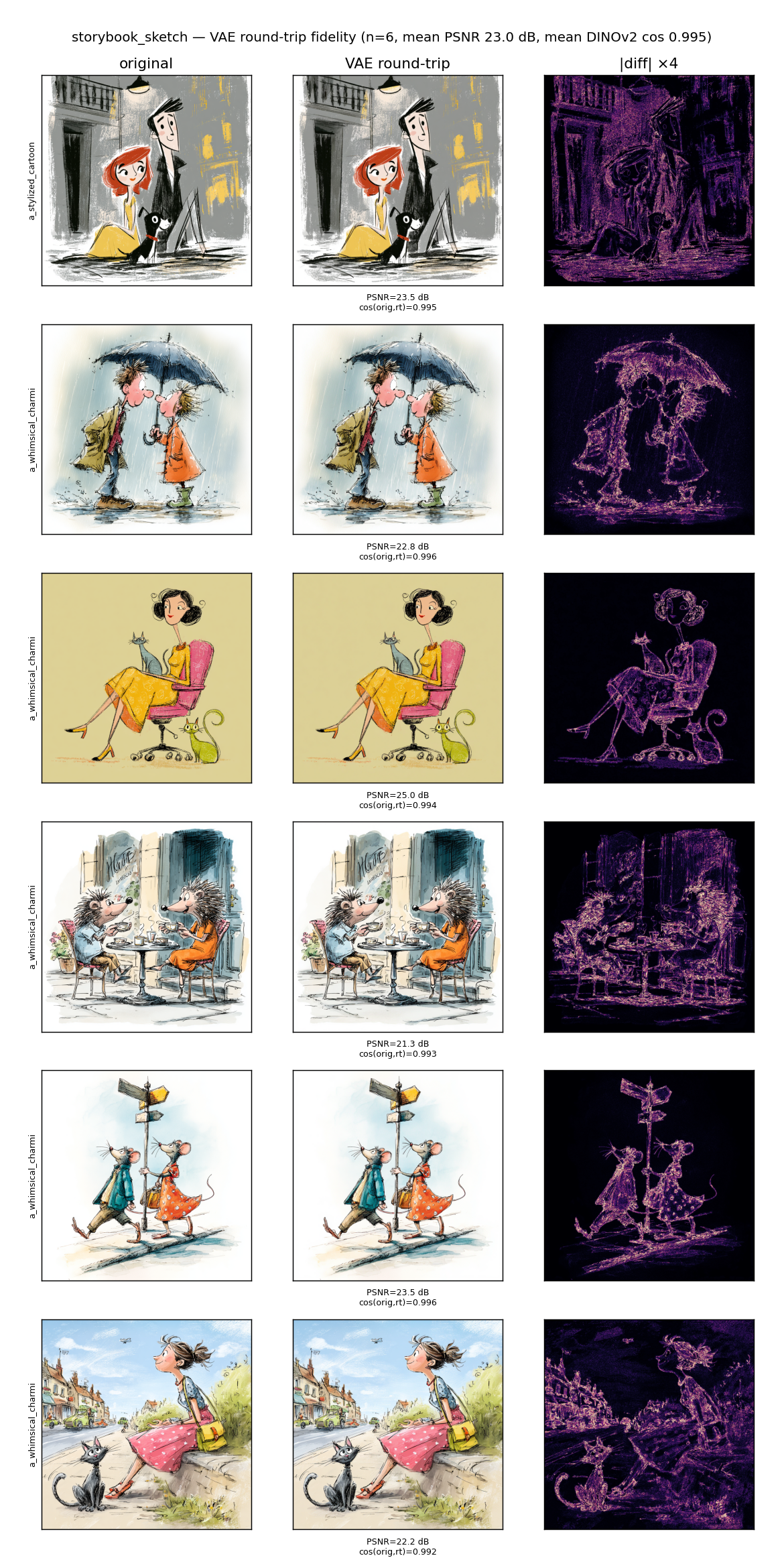
storybook_sketch VAE round-trip (SDXL): the x4 amplified diff glows along the full ink linework (PSNR 23 dB) while the DINOv2 cosine still reads 0.995 — the metric blind spot, demonstrated.

This compounds the scoping above in two ways. First, the headline measurement was the best case: it was taken on ink_wash FLUX (33 dB), but painterly and storybook_sketch ship on SDXL, where comparable content loses 5–8 dB more. The “VAE is unlikely to be the dominant bottleneck” reading is weaker on the platform those styles actually train on, and “cannot be fully eliminated as a contributor to texture loss” is concrete here — a 23 dB round-trip with the linework visibly degraded is a real input-fidelity loss, not a rounding error.

Second, it is the empirical demonstration of the metric blind spot §1 names. On storybook_sketch SDXL the DINOv2 cosine reads 0.9946 — “essentially identical” — while PSNR is 23 dB and the diff shows a large fraction of the high-frequency signal destroyed. The embedding saturates near 1.0 and is blind to exactly the texture loss PSNR and the eye both register. Cosine-to-centroid cannot certify texture preservation; here it visibly fails to — which is why the round-trip verdict rests on PSNR and the amplified diff, not the cosine.

Data integrity: auditing the cached latents

The complement to round-trip fidelity is input-distribution sanity. A data-integrity audit (Figure 9) reads the cached latents as raw tensors (no VAE, no GPU) and flags anomalies in the actual diffusion inputs — NaN/Inf, magnitude outliers (robust median/MAD z-score within each base), near-degenerate / channel-collapsed latents, and foreign-base / bucket mismatches. (This is NOT the DINOv2 style map: the VAE latent is a reconstruction tensor, so its pooled-PCA panel groups by composition/colour, not style — labelled as such.)

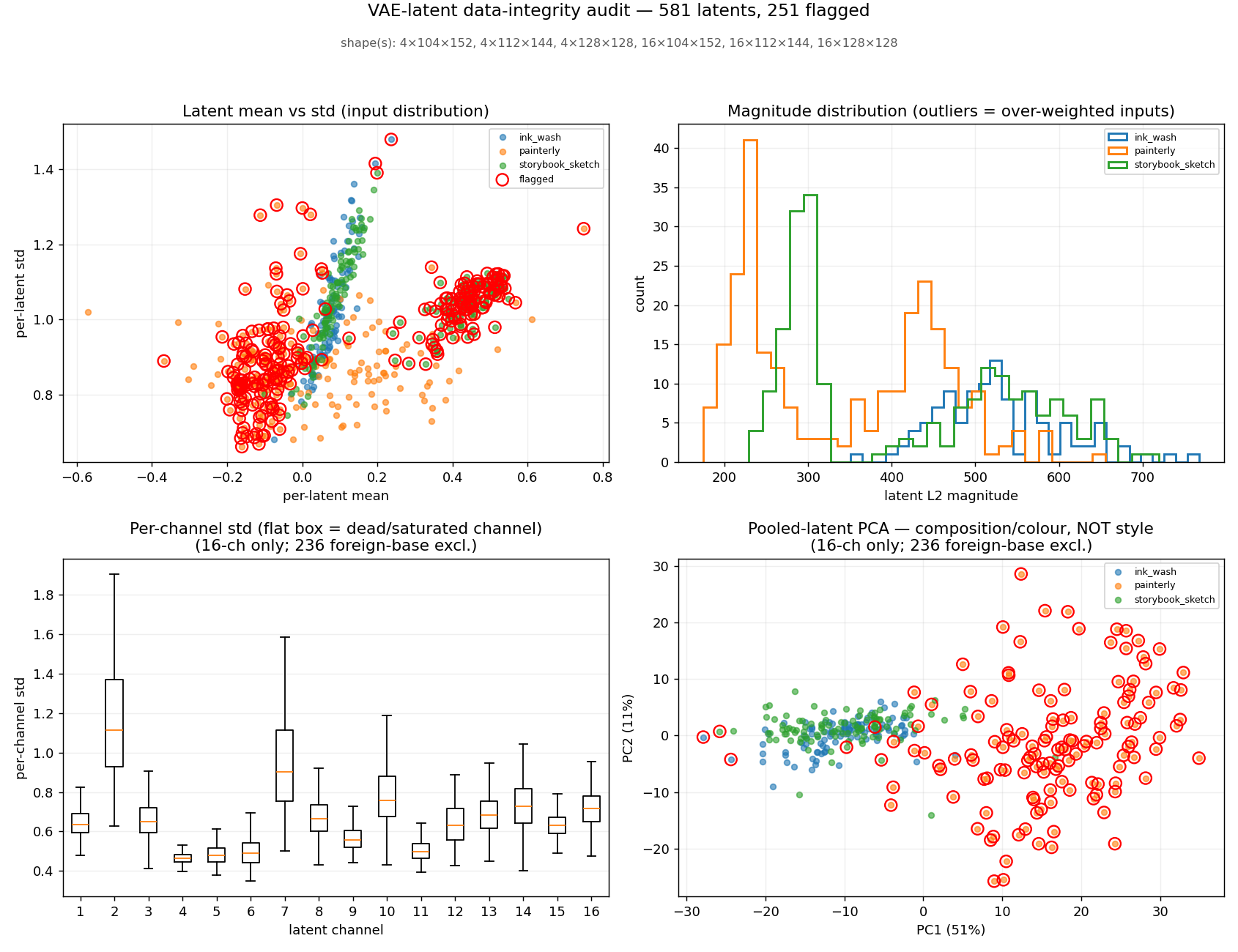
VAE-latent data-integrity audit: per-latent mean-vs-std scatter, L2 magnitude histogram, per-channel std boxplot, and a pooled-latent PCA across the three styles, anomalies ringed. This surfaced the stale mixed-base latents.

It surfaced a cache-hygiene artifact — not a quality bug: painterly and storybook_sketch each carry a matched pair per image — a stale SDXL 4-ch latent left over from the SDXL runs and a fresh FLUX 16-ch latent from a later pass. Because the trainer keys its cache by VAE and loads only the set matching the current base, the stale latents are inert: they never enter training, and ink_wash’s clean all-FLUX cache trains identically. The audit’s value here is the confirmation — no foreign-base latent reached the training inputs, the failure mode it guards against — not a defect it caught. The upshot is housekeeping: clear the latent cache on a base switch to reclaim disk and remove the ambiguity.

---

8. What the LoRA learned: weights, and where they act

§7 verifies the inputs. This reads the trained adapter itself — directly from the weight file, with no base model loaded and nothing generated. A weight audit reconstructs each adapted layer’s update ΔW = B·A and reports, per module: the update magnitude (‖ΔW‖_F), the effective rank of the update (energy-normalised spectral entropy), and how many singular directions hold 90% of its energy. Singular values of B·A come from a small r×r SVD, so the large out×in product is never formed; the audit runs in seconds on CPU.

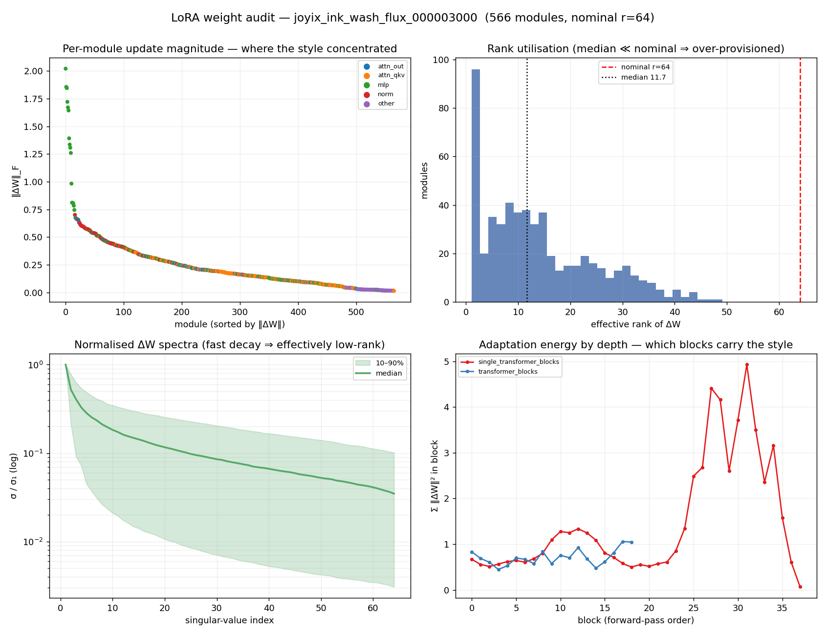
LoRA weight audit, ink_wash FLUX: per-module update magnitude, effective rank vs nominal rank, normalised singular-value spectra, and adaptation energy by block depth — energy spiking in the late single blocks.

For the best ink_wash FLUX LoRA (Figure 10; rank 64, 566 adapted modules):

• Where the style sits. The update concentrates in the MLP projections of the late single-stream transformer blocks (proj_mlp, blocks ~25–35). Single-stream-block MLPs hold 51% of total ‖ΔW‖² across the network, and the top 10 of 566 modules hold 38% of it. The depth panel (bottom-right) shows the energy spiking in the late single blocks while the double-stream blocks stay low — the adaptation is carried by a small, localised set of layers, not spread uniformly.
• How low-rank the update is. A median 19 of 64 directions carry 90% of a module’s energy; the median effective rank is 11.7, the median stable rank 2.4, and the highest-norm MLP layers are near rank-1 (effective rank ~1.5 — one direction holds essentially all their energy). The configured rank 64 sits well above what the update’s energy occupies.

Two levers follow, both of which the eval grid would have to confirm rather than assume: the rank could likely be reduced (low energy-rank is consistent with, but not proof of, no quality loss), and a block-targeted LoRA on the late single-block MLPs would capture most of the adaptation.

Concretely, the energy bounds a rank sweep. The median module fills only ~11–20 of its 64 directions, so:

• rank 48 — pure headroom; the median module wasn’t using 48 directions, so the trim should be lossless.
• rank 32 — ~1.5–3× above the median 90%-energy occupancy (~20 directions); a comfortable margin.
• rank ~24 — roughly at the median 90% line, where the tail of the higher-rank modules starts getting clipped.
• rank 16 — below the median occupancy; expect some loss.

This band is a hypothesis for an eval-grid A/B, not a result. The audit reads the converged ΔW, so it bounds how many directions the final update occupies — not that training at a lower configured rank reaches the same solution. Lower rank constrains the optimisation trajectory, not just the final representation, and an over-parameterised run can locate good directions more easily even when the answer is low-rank. The same-direction evidence is the SDXL run in §9, where dropping ink_wash from rank 128→64 lifted the mean (+0.029, less overfit) rather than hurting it — but that was a different base that stopped at 64, so the sub-64 FLUX trim earns its own sweep (fixed training seed, lowest rank still within the noise band of rank 64).

The same structure on SDXL — and on a standard dataset

The FLUX finding has a clean SDXL analogue, and it holds on the standard naruto-blip-captions set (nrtcel) as much as on the project’s own sub-styles — so it is not an artifact of the custom data. The same audit, reading the SDXL UNet’s down→mid→up blocks (Figure 11):

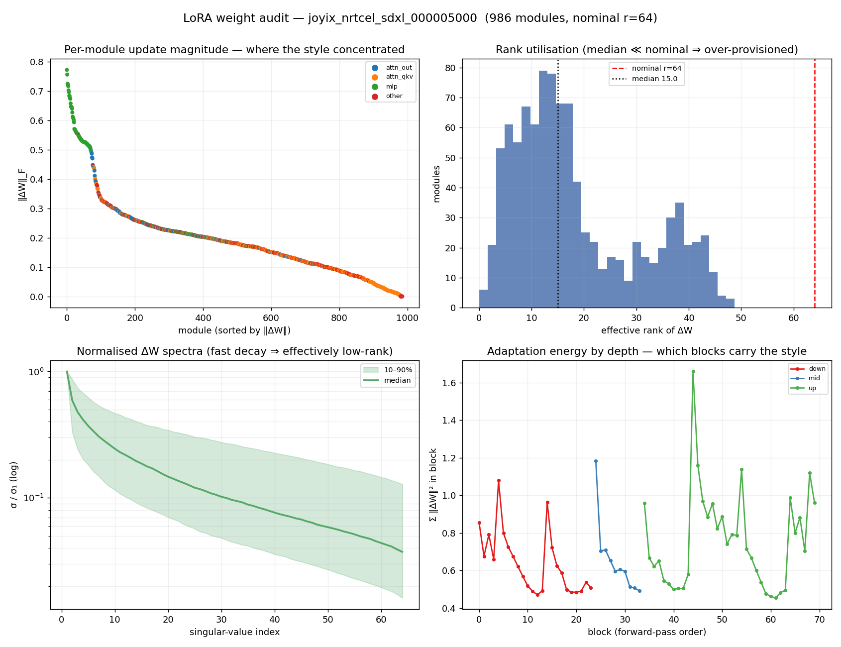
SDXL weight audit, nrtcel (the standard naruto-blip-captions set): magnitude, rank utilisation, spectra, and energy by UNet depth — the up (decoder) blocks carry the style.

SDXL sub-style	rank	up-block-MLP share of ‖ΔW‖²	median eff-rank
nrtcel (standard)	64	26.8%	15.0 / 64
painterly	128	29.9%	24.7 / 128
storybook_sketch	64	34.3%	14.1 / 64

In all three (Table 5) the up (decoder) block MLPs are the single largest energy bucket — the SDXL counterpart of FLUX’s late single-block MLPs — and the update is low-rank (median ~20–30% of the nominal rank). So the cross-architecture rule is the same: the style rides on the MLP / feed-forward projections of the late, decoder half of the network, in a handful of low-rank directions — not on attention, not on early layers. The standard dataset behaves exactly like the bespoke ones. (nrtcel and storybook_sketch are both rank 64 — their median eff-ranks, 15.0 and 14.1 of 64, are directly comparable, and storybook concentrates a little more in the up-MLPs; painterly is shown at rank 128, the rank it ships at, so its 24.7/128 isn’t on the same axis, but its up-MLP concentration and low utilisation match regardless. Each style’s audit reads the tensor it ships — §9; painterly and storybook_sketch are Figures 12–13.)

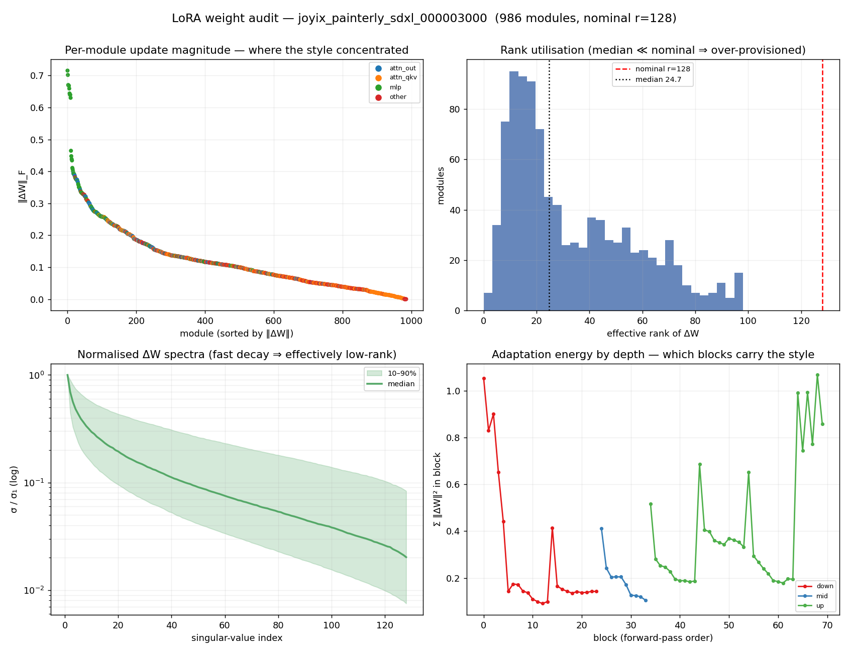
painterly SDXL weight audit — same shape: the up-block MLPs dominate, in a handful of low-rank directions.

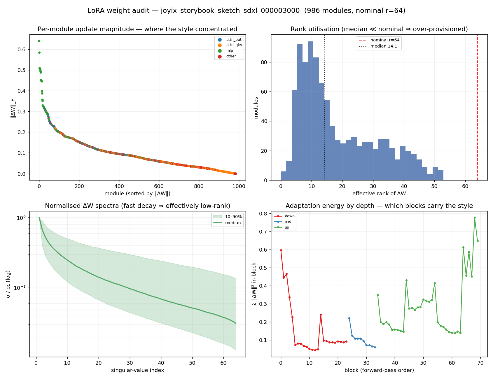
storybook_sketch SDXL weight audit (rank 64, its shipped tensor) — same shape: up-block MLPs dominate, low effective rank.

Why the FLUX spectra band is wider — architecture, not data

The normalised-spectra panel (bottom-left of each audit figure) shades the 10–90% band of σ_i/σ₁ across modules; its width is module-to-module heterogeneity in decay shape — wide ⇒ some modules are near rank-1 while others stay nearly flat. The FLUX panel shows a visibly wider band than any of the SDXL panels (Figure 14), and it is worth settling what that reflects. Reducing each adapter to one comparable scalar — the mean band width over fractional rank positions (5/10/25/50%, so a rank-64 and a rank-128 adapter share the same relative axis) (Table 6):

LoRA	base	rank	band width	eff-rank range (p10 → p90)	CoV
ink_wash	FLUX	64	1.18 dec	1.5 → 30.8 (min 1.1, max 49.2)	0.76
nrtcel	SDXL	64	0.62 dec	5.4 → 38.2	0.65
painterly	SDXL	128	0.67 dec	9.4 → 69.1	0.71
storybook_sketch	SDXL	64	0.62 dec	5.7 → 39.4	0.68

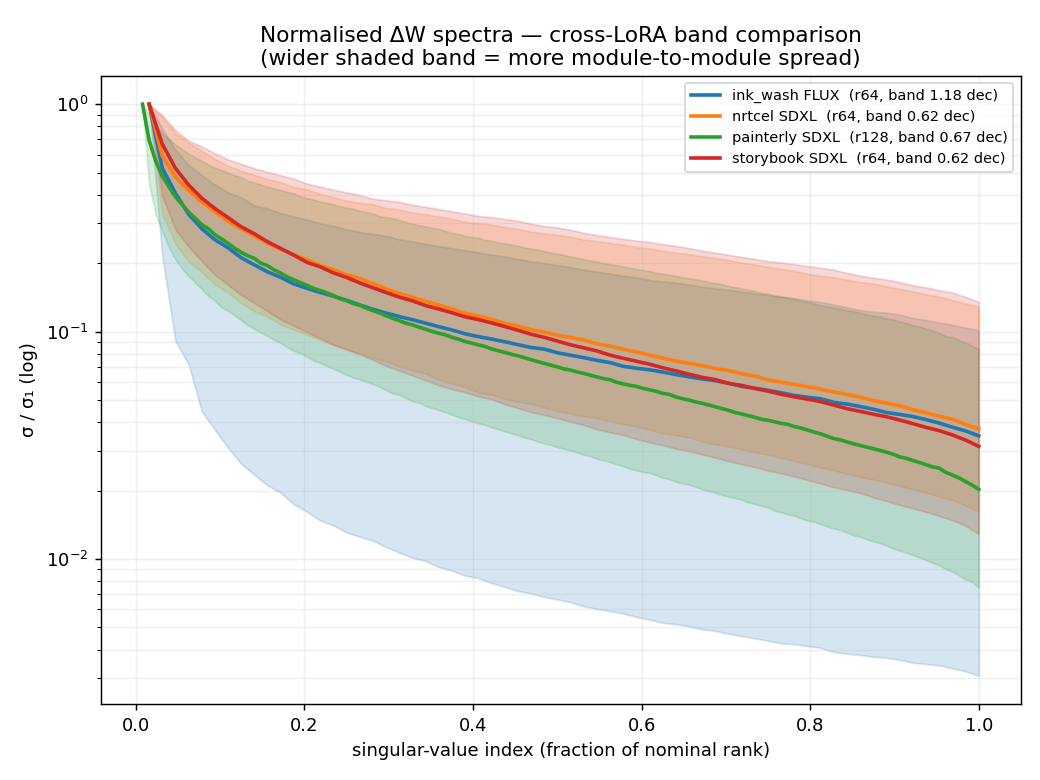
Cross-LoRA normalised ΔW spectra with their 10–90% bands, index axis as a fraction of nominal rank so ranks align. The FLUX band is roughly twice as wide as every SDXL band while the median curves nearly coincide — architecture, not data.

Three factors separate cleanly:

• It is the base model. At matched rank 64 the FLUX band (1.18 dec) is about twice every SDXL band (0.62 dec). Holding rank fixed isolates the architecture.
• It is not the data. Two unrelated SDXL datasets at the same rank 64 — a public character set and a bespoke style — land at an identical 0.62 dec. The style being adapted barely moves the spread.
• It is not mainly the rank. The same dataset at both ranks settles it: storybook_sketch spreads 0.62 dec at rank 64 and 0.69 at rank 128 — a ~0.07 widening for doubling the rank, an order of magnitude below the FLUX–SDXL gap (painterly, at rank 128, sits at 0.67). Rank lengthens the index axis without much stretching the band.

The mechanism is the floor of the effective-rank distribution. SDXL’s lowest-rank modules bottom out around eff-rank 5–9 (the p10 column); FLUX’s p10 is 1.5, with a population of modules that are essentially rank-1 — one singular direction holds nearly all of that module’s ΔW energy, so σ₂/σ₁ collapses and the module sits a full decade below the median, pulling the bottom of the band down. Those near-rank-1 modules are the same high-energy late single-block feed-forward projections identified above, and they coexist in one network with higher-rank attention projections (up to eff-rank ~49). A module population spanning rank-1 to rank-49 is what stretches the band; SDXL’s UNet drives no module that close to rank-1, so its per-module curves bunch together and its band stays narrow. The median curves themselves sit close together across both bases (median σ/σ₁ ≈ 0.06–0.10 at the half-rank index), so the difference is dispersion, not a faster average decay.

This is also a reading caution for the panels above: the FLUX figure and the SDXL figures differ in base, dataset, and (for two of them) rank at once, so the wider FLUX band reflects architectural module heterogeneity — not ink_wash being intrinsically harder or more rank-hungry than the SDXL styles.

The audit says where and how much the weights moved; it does not say what visual feature each direction encodes, or where on the canvas the style acts. The next probe addresses the “where.”

Where the trigger acts — and what a baseline reveals

The weight audit is static — it reads the adapter at rest. To see what happens at generation time, a DAAM-style probe records, during a real generation, how much each image position attends to each text token (the diffusion counterpart of a saliency map), and overlays that per-token heatmap on the output. The probe loads the full adapter (both the UNet and the text-encoder halves) and renders with the production sampler recipe, so its image tracks normal output rather than drifting toward a washed-out render; the attention pattern is the result either way (Figure 15).

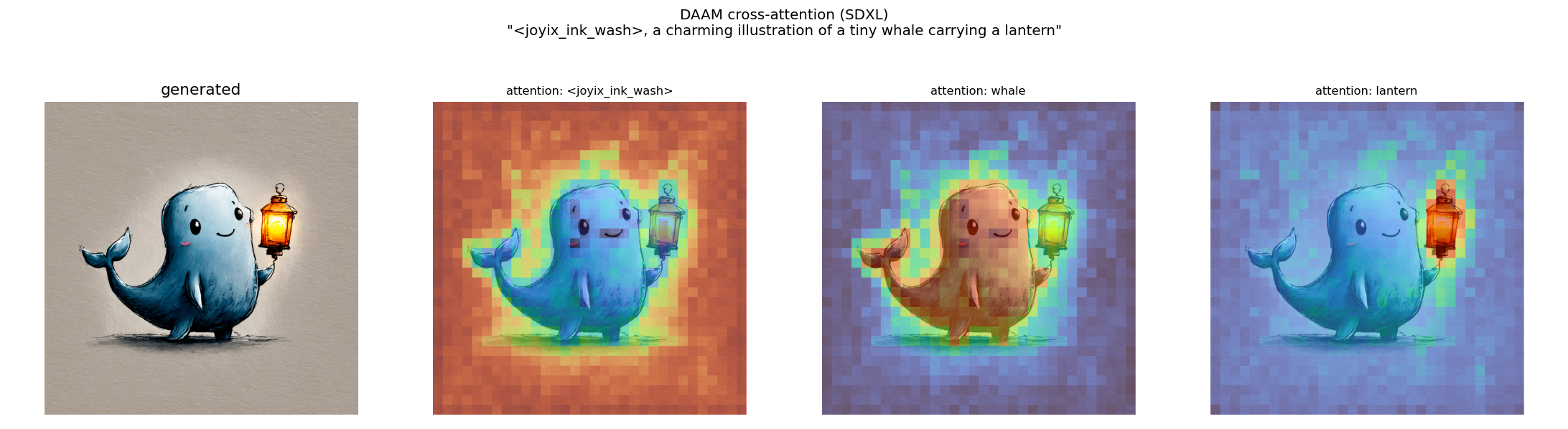
SDXL attention attribution, LoRA on: the whale-with-lantern generation, then per-token heatmaps — content words land on their objects, the trigger is diffuse.

Two things show up: content words — whale, lantern (and on FLUX, birds, branch) — concentrate on their objects, and the trigger token is diffuse. The tempting reading is “the trigger learned to control the whole-image style.” A baseline control settles whether that’s true: run the same probe with the LoRA turned off (scale 0). The attribution barely moves (Table 7) —

token	LoRA off	LoRA on
trigger token	48%	47%
whale	40%	38%
lantern	48%	48%

(mass-50%-area; higher = more spread; identical seed/steps/size). With and without the LoRA the trigger is equally diffuse and the content words equally localised — only the rendered style changes (the LoRA-off image is plain base-model, not ink-wash) (Figure 16):

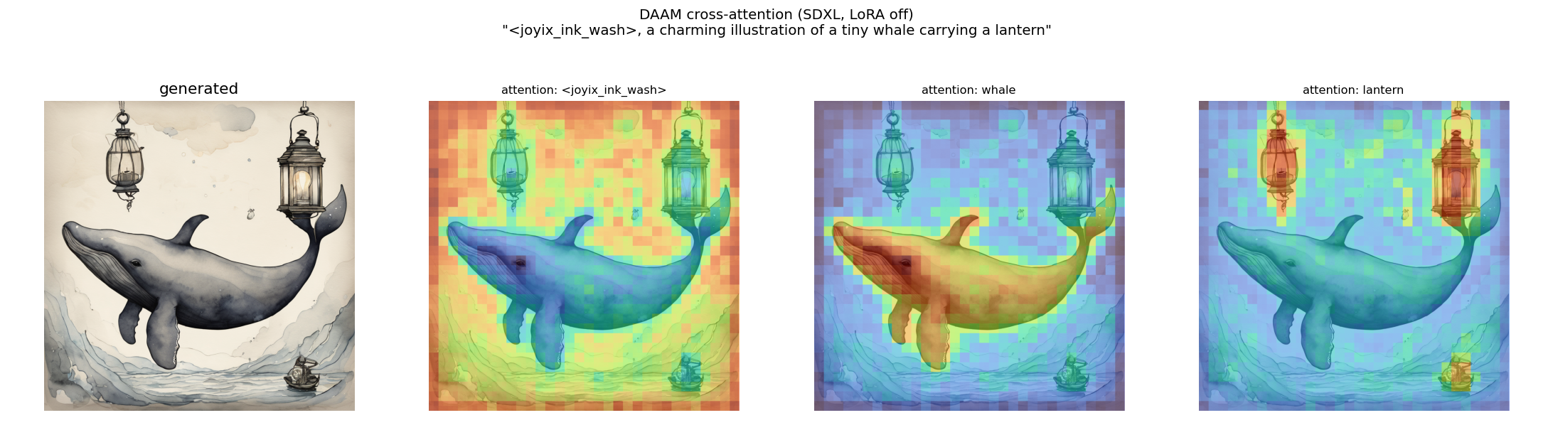
The same prompt with the LoRA off (baseline): near-identical attention maps — only the rendered style changes. Without this control, the diffuse trigger map reads as a finding; with it, the finding evaporates.

So the honest conclusion is the opposite of the tempting one: a style LoRA’s effect is largely invisible to attention attribution. Cross-attention attribution reflects semantic layout — which region cares about which word — and a style LoRA changes appearance, not semantics. Content words localise because the base model already knows them; the trigger is diffuse because it is an uninformative multi-subword token that attracts sink-like attention — both true with or without the LoRA. The trigger’s spread is not evidence of a learned global-style role.

The pattern is not specific to ink_wash. Running the identical on/off probe on the other two SDXL sub-styles — same prompt (a mouse in a top hat at a tea table), same seed — reproduces it: the per-token maps barely move between LoRA-on and LoRA-off, while only the rendered medium changes. For painterly, the LoRA turns a plain base render into oil-brush colour; the trigger stays diffuse and mouse / table / hat stay pinned to their objects either way (Figures 17–18):

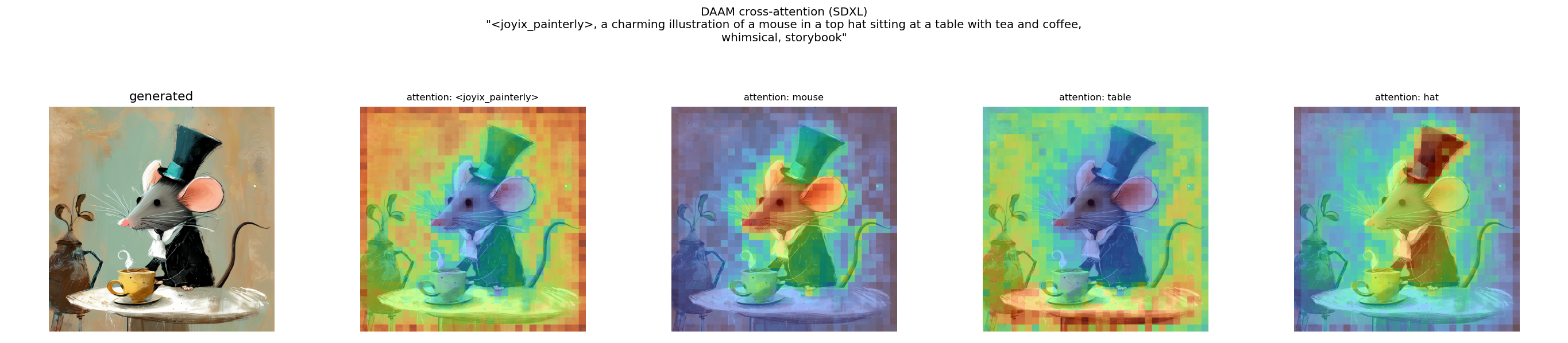
painterly SDXL attention attribution, LoRA on: an oil-painterly mouse in a top hat — trigger diffuse, mouse/table/hat localised.

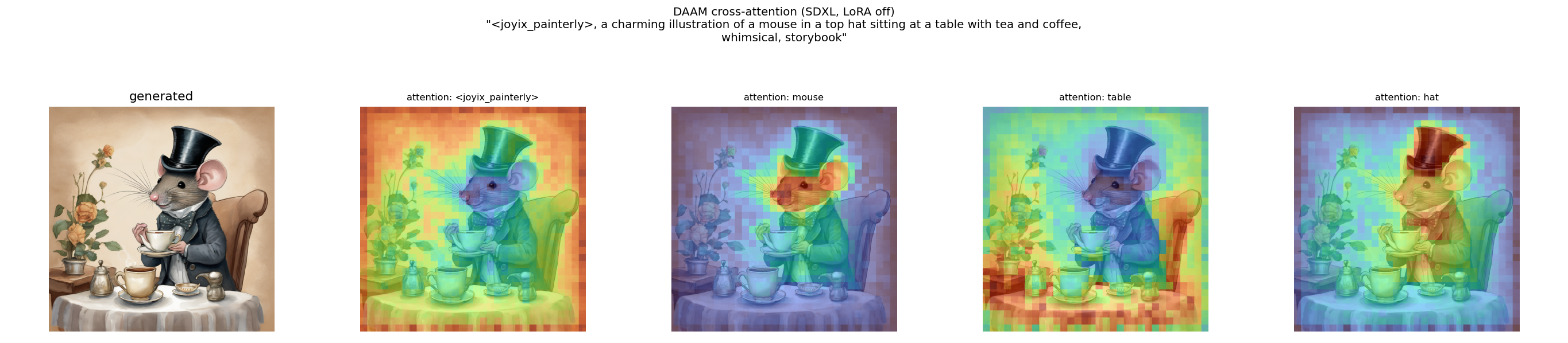
painterly, LoRA off (baseline): the same prompt in plain base-model style, with near-identical attention maps.

For storybook_sketch, the LoRA swaps the same base scene for pen-and-ink line work — and again the attribution is unchanged, only the medium (Figures 19–20):

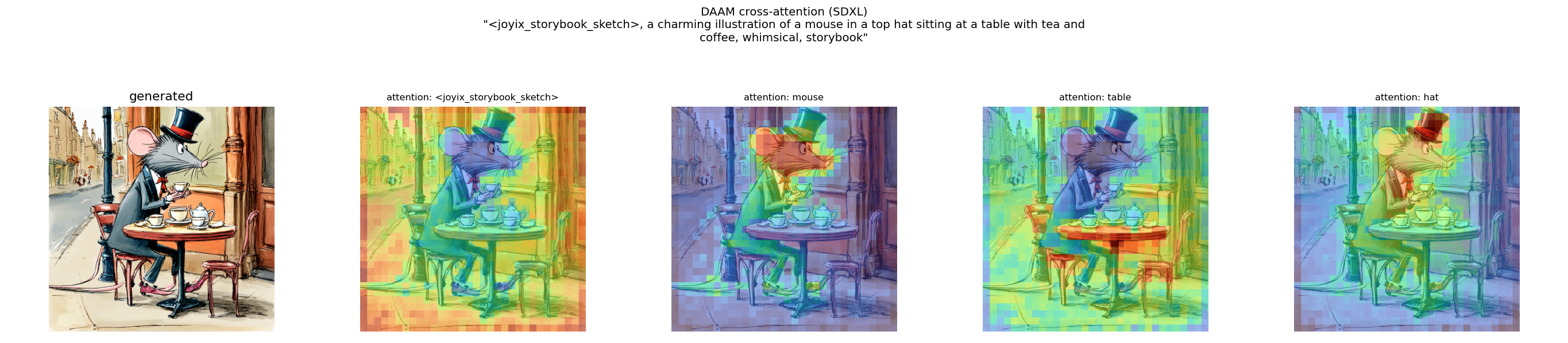
storybook_sketch SDXL attention attribution, LoRA on: a pen-and-ink storybook mouse — trigger diffuse, mouse/table/hat localised.

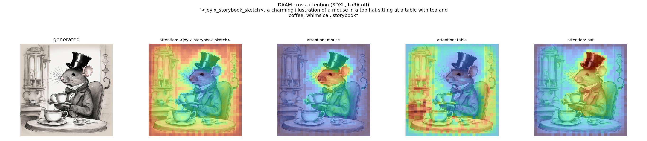
storybook_sketch, LoRA off (baseline): the same prompt in plain base-model style, with near-identical attention maps.

The probe is still good for one thing — confirming that content tokens land on their objects, a clean check that prompt and image align. It works identically on FLUX, whose MMDiT joint attention needs a different extraction (intercepting the joint attention and isolating the image→text block; all 57 attention layers × every step were captured); there birds and branch localise even more sharply (Figure 21):

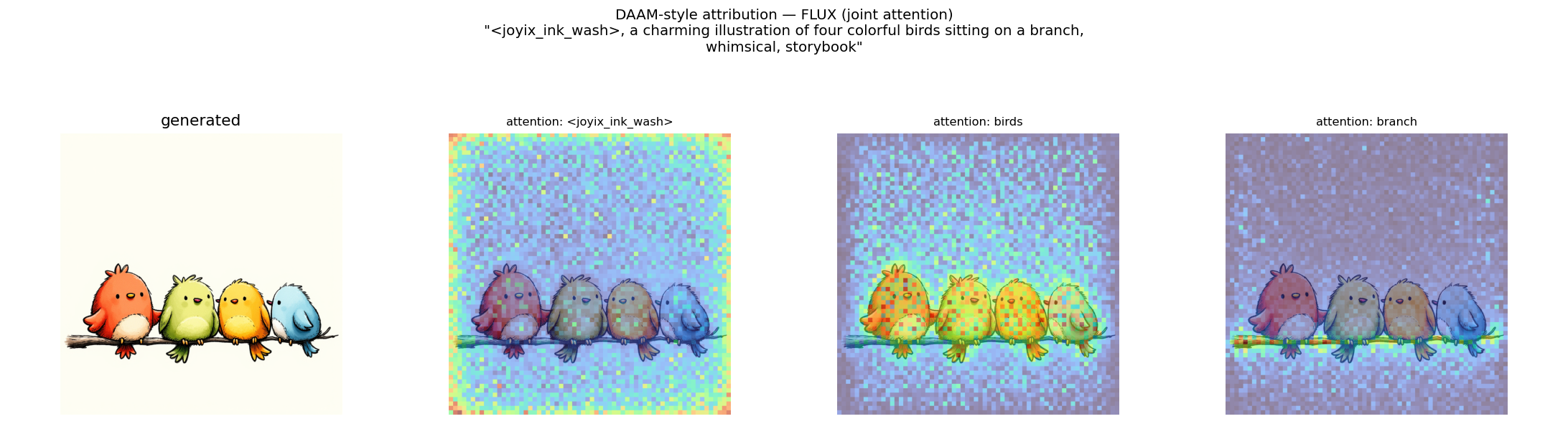
FLUX attention attribution (joint MMDiT attention): four birds on a branch — ‘birds’ on the birds, ‘branch’ along the branch, trigger diffuse.

The same off-switch closes the loop on FLUX too: with the LoRA off the birds render in plain base style, yet birds and branch land in the same places — the attribution is a property of the base model’s joint attention, not the style adapter (Figure 22):

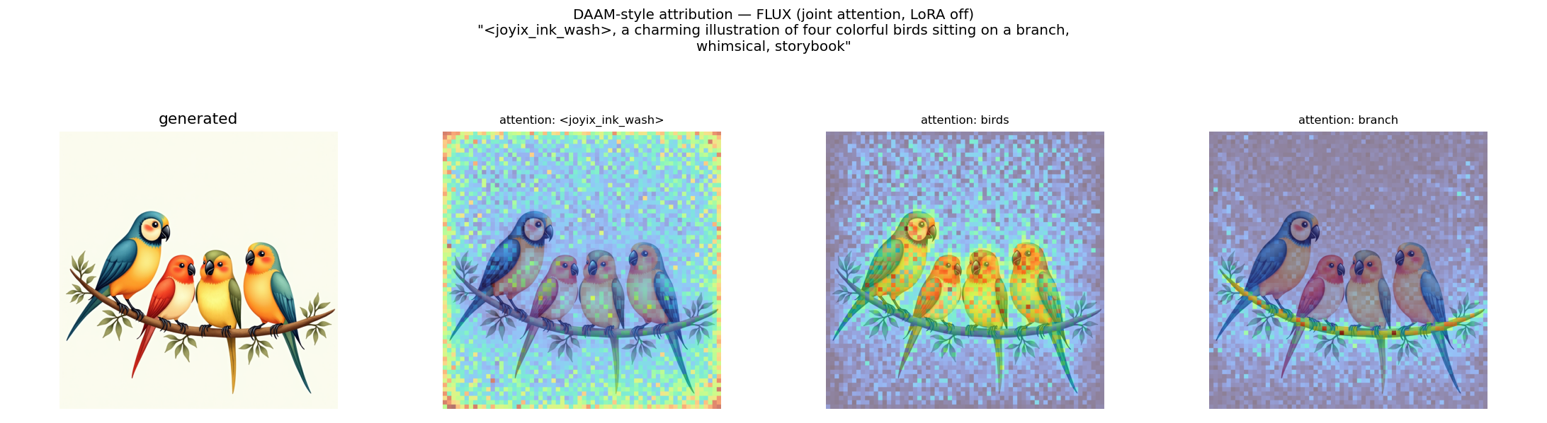
FLUX, LoRA off (baseline): the same birds/branch localisation in plain base style — the attribution is a property of the base model’s joint attention, not the style adapter.

But for understanding what a style LoRA learned, attention attribution is the wrong lens — the weight audit above and the perceptual DINOv2 metric (§5) are the right ones. The real lesson is about the baseline: without it, the diffuse trigger map reads as a finding; with it, the finding evaporates. (FLUX runs on the larger training hardware; SDXL — including the LoRA-on/off A/B above — runs on a single consumer card.)

---

9. SDXL results across all three sub-styles

SDXL is the workhorse platform; all three styles were trained and evaluated on it first. All numbers are best-checkpoint, in-domain, 2-seed mean (best step selected per style/seed on the stable mean, then averaged over two training seeds). gate is each folder’s calibrated p25 (§3). The per-style picture (Table 8):

sub-style	best-ckpt (per seed)	mean	gate	margin	rate	memo
painterly	s1:step3500 / s2:step3000	0.575	0.556	+0.018	66% (peak 73%)	0%
storybook_sketch	s1:step4000 / s2:step5000	0.635	0.629	+0.006	53%	0%
ink_wash (213, rank 128)	s1:step4500 / s2:step2500	0.609	0.659	−0.050	42%	0%

Reads:

• All three underfit the 90% rate bar — none is “done” on SDXL.
• painterly and storybook clear their gate on the mean (positive margin) but still miss the rate bar — their output distribution sits on the gate, so the rate is a coin-flip (§5.1). They need a small push, not a platform change. painterly’s free win is pure checkpoint selection: ~66% at its best step vs 49% at final.
• ink_wash is the outlier — the only style whose best checkpoint mean sits below its (highest) gate. It became the priority and the deep-dive subject.

ink_wash SDXL — isolating set size vs rank

ink_wash was reduced from a 213-image set to a deliberate 109-image variety pick (subject/design diversity at one consistent style — not a random subset). Its intra-set stats nearly match the 213 (mean 0.701 vs 0.710, p25 0.658 ≈ 0.659), so it’s scored against its own folder and stays directly comparable to the 213 baseline with no restore-to-213 needed (Table 9):

variant	set / rank	mean	gate	margin	rate	memo
baseline	213 / rank 128	0.609	0.659	−0.050	42%	0%
set-size only	109 / rank 128	0.615	0.658	−0.043	42%	0%
+ rank 64	109 / rank 64	0.644	0.658	−0.014	47%	0%

Verdict: set size is NOT the lever; rank is. At matched rank 128 the 109 set only ties the 213 baseline (0.615 vs 0.609, within the noise band) — the “smaller set = more per-image exposure = better” hypothesis is false. Dropping rank 128 → 64 on the 109 set is what lifts the best-checkpoint mean to 0.644 (+0.035 over baseline) with memo still 0%: lower adapter capacity = less overfit on the smaller set. This is the best honest ink_wash SDXL result — but still −0.014 under gate and 47% ≪ 90%. (A separate 31-image flat-texture-curation probe, sktchyInk, cleared its own gate but memorized 13–19% and only tied 109+rank64 on the common bar — the curation principle transfers, the tiny set overfits.)

The standard-dataset run in §5 supplies the complement, and it flips the sign: nrtcel (1107 images, ~10× ink_wash) is better at rank 64 than rank 32 — at matched eval prompts, 0.666 vs 0.602 (+0.064), and the gap holds at matched step, so it’s a rank effect not a step-count one. (Prompt-set sensitivity on that comparison was ~0.008 — the same rank-64 LoRA scored 0.658 vs 0.666 on two independently-derived 50-subject sets — an order of magnitude below the rank effect, so it isn’t a prompt artifact.) So “lower rank wins” is not a law. The ink_wash↔nrtcel contrast reads as match rank to set size — a small set (109) overfits the extra capacity so dropping rank helps; a large, genuinely varied set (1107) uses it so raising rank helps. But set size turns out to be only a loose proxy for the real variable, as two more small sets show next.

Two more small sets: the rank reduction does not generalize uniformly

If the rule were strictly set size, painterly (~130 images) and storybook_sketch (~106) — both small — should both improve at rank 64 the way ink_wash did. Each was re-trained at rank 64 and scored on the same committed in-domain prompt set and gate as the rank-128 runs. Two of the four rank-128 runs share their training seed with the rank-64 runs — a within-seed A/B where rank is the only variable — while the other two widen the rank-128 sample. Reading both the controlled within-seed Δ and the full rank-128 seed range against the rank-64 one, neither small set reproduces the ink_wash win (Table 10):

sub-style	rank-128 (mean, range; n)	rank-64 (mean, range; n)	within-seed Δ
painterly	0.572, 0.550–0.600 (4)	0.561, 0.559–0.562 (2)	−0.025, +0.006
storybook_sketch	0.639, 0.632–0.643 (4)	0.647, 0.645–0.649 (2)	+0.004, +0.006

Best-checkpoint in-domain mean; within-seed Δ is rank-64 minus rank-128 on each of the two shared seeds.

• painterly shows no reliable rank effect. Its rank-64 runs (0.559–0.562) sit inside the far wider rank-128 seed range (0.550–0.600) — no separation — and the two within-seed deltas disagree on sign (−0.025 and +0.006), so the apparent rank-64 penalty is one seed, not a trend. What rank 64 does do is collapse the seed spread, 0.050 → 0.003: lower capacity is more seed-stable, but at the same mean, not a higher one.
• storybook_sketch mildly prefers rank 64. Both rank-64 runs (0.645, 0.649) clear every one of the four rank-128 runs (top 0.643), and both within-seed deltas are positive (+0.004, +0.006) — +0.005 on the seed-matched mean. A clean separation, but a small one, at the prompt-set noise floor.

Three small sets, three answers: ink_wash gains clearly at rank 64 (+0.029), storybook marginally (+0.005), painterly not at all (a seed-volatile wash). So the operative variable is not set size — all three are small — but how much genuine variation a set carries, i.e. how much adapter capacity the style actually uses. The lever is still rank; the honest rule is match rank to the variation the data carries, for which set size is only a rough stand-in. A single set’s rank-64 win does not transfer on size alone.

The shared wall: ~0% diversity on all three

Held-out novel-subject prompts (the 5-prompt tail), per-image DINOv2 vs the relaxed p10 gate (Table 11):

sub-style	diversity sims (5)	p10 gate	rate
ink_wash	0.56, 0.44, 0.38, 0.57, 0.51	0.614	0%
painterly	0.29, 0.21, 0.42, 0.43, 0.33	~0.50	0%
storybook_sketch	0.51, 0.47, 0.32, 0.46, 0.36	~0.58	0%

All three collapse to ~0% on novel subjects — a uniform out-of-domain generalization gap that no recipe knob fixes. These folders pass the caption-diversity audit (no single subject family dominates), yet still collapse out-of-domain — so the lever is broader reference + caption subject coverage (§6, the data lever), not a recipe change. This is the clean empirical separation of the two failure modes: in-domain underfit moved with rank; the diversity wall did not move with any recipe knob.

---

10. FLUX (ink_wash) — the recipe frontier

FLUX is the hero-quality platform but was the last lever, run only after the cheap SDXL levers stalled, and judged on the same mean/margin bar — never promoted on its “hero model” reputation (Table 12):

variant	mean	gate	margin	rate	note
FLUX, freeze-TE, no descriptor	0.568	0.658	−0.091	21%	decisively worse than SDXL (then)
FLUX + TE-LR fix + descriptor@inference (seed_42)	0.668	0.658	+0.010	67%	clears gate; beats SDXL 0.644
FLUX, same recipe, seed_77	0.583	0.658	−0.075	—	same recipe, ±0.085 worse
FLUX, descriptor in training (seed_42)	0.612	0.658	−0.046	—	regression → §4

Two interventions un-shelved FLUX from 0.568 to ~0.67:

1. TE-LR fix — a small tracked patch to the trainer, pinned to a specific upstream commit, that wires up the parsed-but-ignored per-group learning rates (set text_encoder_lr 1e-5 / unet_lr 1e-4) and routes the warmup-step count through the scheduler (stock behaviour silently defaulted warmup to 1000 steps and ignored it for cosine entirely). The recipe you think you’re running was not the one that ran — see §11.
2. Textured-paper descriptor at inference (NOT in training — the descriptor-in-training A/B in §4 shows that regresses it).

But the dominant variable turned out to be the training seed: the ~0.085 seed_42↔seed_77 gap persists across every generation-seed (§6), ~4× the eval noise. So FLUX with the right seed beats the SDXL platform (+0.024 over 0.644) — but a single seed lands ±0.085 apart, making best-of-N training-seed selection mandatory. Even the best seed only clears its own gate by +0.010 (short of the strict +0.02 adopt line) and still fails the 90% rate + 0% diversity. ink_wash is shelved at the ~0.67 ceiling — a cost/priority call, with the untouched data lever (§9) the remaining frontier, not a proven hard ceiling.

---

11. The architectural finding that bounded the recipe frontier

On FLUX, the trainer’s text-encoder LoRA targets only the CLIP attention / MLP modules, so it adapts CLIP-L only; T5-XXL stays frozen (it only touches T5 for a different architecture). This is verified in the trainer’s source — and the diffusers reference FLUX LoRA script does the same under --train_text_encoder, so it’s a platform convention, not a trainer quirk. Implications, given the results:

• The TE “win” is a global pooled-style-vector shift (CLIP-L feeds FLUX’s AdaLN modulation), not per-word binding (T5, which carries the detailed semantics, is untouched).
• This predicts the descriptor-in-training regression (§4): you cannot bind texture into frozen-T5 descriptor tokens, so naming it only steals ownership from the trigger.
• It decouples the TE lever from the diversity hole (the semantics encoder isn’t trained) → the 0% diversity is a data problem, confirming §9’s split.

Two trainer-internals corollaries that changed what actually ran: the per-group learning rates (text_encoder_lr / unet_lr) were parsed but never read (both groups hardcoded to the single base LR), and the warmup-step count was silently ignored. Both are fixed by the tracked patch (§10). The lesson: know your trainer’s internals — the recipe you configure may not be the recipe that executes.

---

12. What generalizes (the transferable checklist)

1. Pick a style-dominant embedder (DINOv2 — strongly style-weighted, though not subject-invariant) and use it for everything — triage, curation, eval. One feature space = “passes triage” and “passes eval” mean the same thing. Because it stays entangled with subject and layout, gate on it relatively (same-subject distribution, mean over many images), never as an absolute per-image style score.
2. Calibrate every gate to the dataset’s own distribution (per-folder p25 / p10), never a guessed absolute. (Three styles → three gates: 0.556 / 0.629 / 0.658.)
3. Gate coherence before you train — move detection upstream of GPU spend; let a non-zero pre-flight halt the run.
4. Captions: build forward from bare subjects; caption what varies, omit what the trigger owns. Freeze the inference prompt per-LoRA to kill drift. And validate the subject tier — a public dataset’s captions are unvalidated input (“on a model hub” ≠ checked), and the build propagates a wrong subject faithfully.
5. Grade on the mean at the best checkpoint, in-domain, with the diversity tail scored separately at a relaxed gate.
6. Treat the noise band as a number. Pre-declare an adopt threshold (> 0.02 over gate). Separate training-seed effect from eval noise with a sweep.
7. Separate the two failure modes (in-domain underfit = recipe; out-of-domain = data) and map each lever to the mode it can actually move.
8. Know your trainer’s internals — per-group LR and warmup were silently ignored; the FLUX TE-LoRA is CLIP-L-only. The recipe you think you’re running may not be the one that ran.

---

13. Tooling landscape: what exists, what’s missing

The diagnostics here are assembled from techniques that already exist across ML, not invented for this project. This section is a map of what is and isn’t routinely available, so the gaps are explicit and so anyone wanting to go further knows what to read.

What general-purpose LoRA training frameworks expose today (kohya_ss / sd-scripts, ai-toolkit, OneTrainer, the diffusers training scripts): training-loss scalars, periodic sample images at fixed prompts, and basic TensorBoard logging. The diffusion training loss is a weak quality signal — it’s averaged over random timesteps and noise levels, so it barely tracks sample quality — which is why the working signal in practice is eyeballing the sample images. Rank, LR, and steps are set by convention.

What exists in research / adjacent tooling but is rarely wired into LoRA training:

• Attribution / interpretability: DAAM (cross-attention attribution — a spatial saliency map per prompt token), attention rollout, Prompt-to-Prompt — the diffusion analog of Grad-CAM, mapping a generation back onto the tokens and regions that drove it.
• Adapter analysis: SVD / spectral analysis of the LoRA update (AdaLoRA allocates rank by singular-value importance); block-wise LoRA weighting (per-block rank / LR). The §8 weight audit is in this family.
• Data quality: confident-learning and data auditing (cleanlab), data-validation frameworks (TFX Data Validation, Great Expectations), dataset cartography. The §2–§3 curation gate and the §7 latent audit are in this family.
• Generative evaluation: learned human-preference models (HPSv2, ImageReward, PickScore) and distributional metrics (FID, CLIP-score). The §5 DINOv2 gate is a dataset-relative instance of this idea.
• Style representation: Gram-matrix / VGG style statistics (the classic neural-style-transfer signal) as a second, mechanistically independent style metric.

What is missing as routine LoRA-training diagnostics — candidate additions to a framework:

• a post-train weight report (effective rank per layer, ΔW by block) to inform rank and block-targeting (§8);
• dataset-relative on-style gating instead of fixed similarity thresholds (§3);
• input-integrity checks on the latent cache — corrupt / anomalous / mixed-base latents (§7);
• held-out generalization and memorization numbers emitted as standard train outputs (§5–§6), rather than inferred from sample grids;
• activation / attention attribution wired into the sample previews, so a preview answers “where did the trigger act,” not only “does it look right.”

The individual pieces are established and well-documented; the aim here is just to gather them in one place and run them as part of a LoRA train, in case that’s a useful starting point for someone learning the same thing. The attribution row above (DAAM-style) is built and verified on both SDXL and FLUX (§8) — and a baseline control there shows it reflects semantic layout, not the style LoRA, so it reads content-token localisation but not the style itself.

---

Reproducibility & method notes

Every figure and number above is read back, by small reader scripts, from artifacts saved at generation time — none is hand-tuned for the writeup. In brief:

• Eval numbers (the SDXL/FLUX best-checkpoint tables) come from the per-image DINOv2 scores stored in each eval run’s report, re-aggregated to the best-checkpoint, in-domain, 2-seed mean. Scoring is independent of generation, so reports are re-readable — and correctable — without regenerating images.
• Calibrated gates are the per-folder p25 of the reference set’s intra-set DINOv2 cosine distribution (§3).
• Reference-distribution figures (ridgeline, 2-D embedding map, separability table) are pure readers over the cached DINOv2 embeddings — no GPU, no re-embed.
• VAE round-trip decodes the cached training latents through the local VAE and compares to the originals (PSNR + DINOv2 cosine); the latent data-integrity audit reads the same latents as raw tensors (no VAE, no GPU).
• The weight audit (§8) reads the trained LoRA’s weight file directly and reconstructs each layer’s update ΔW = B·A; its singular values come from a small r×r SVD, so the base model is never loaded.
• Two external-code findings are load-bearing: the trainer’s text-encoder LoRA targets only the CLIP attention / MLP modules, so on FLUX it adapts CLIP-L and leaves T5 frozen (§11); and a small tracked patch fixes the trainer’s per-group learning-rate and warmup handling (§10), pinned to a specific upstream commit so the fix is reproducible.